Modern Storage Systems
January 2020
This post is a draft. Content may be incomplete or missing.
Did you know there’s a small set of basic data structures and algorithms that underpin just about every software system that stores and retrieves data on disk, from databases to file systems and more?
There’s a fairly straightforward line of reasoning that you can follow to get more or less to today’s state of the art — all you need is some basic familiarity with data structures like hash tables and binary trees. That lines of reasoning goes something like this:
Let’s Design a Store
We’ll start with one of the most basic kinds of storage systems: a key/value store, where we store both the keys and values on disk with the following interface:
- The client (our user) defines the structure of a key and a value
- Our write method adds a key/value pair to add to our store
- Our read method accepts a key, and reads the corresponding value from the store
This interface should seem familiar: it’s the basic key/value map interface provided by many programming languages and runtimes. If this seems like an odd interface to use for disk storage, keep in mind that most “real” storage systems rely on something that looks an awful lot like a key/value mapping, even if these systems don’t specifically use the words key and value. For example:
- Want to open a web page? You need to provide its URL (a key)
- Want to read a file? You need to provide its path (a key)
- Want to load a value from memory? You need to provide its address (a key)
- Want to query a database? You need to provide a primary key
Later on we’ll see how to gussy up an on-disk key/value store like this one to make it the core of a database, a file system, or maybe something else. But for now let’s focus on how to build a store like this one efficiently.
The Key Problem
When designing something, a good question to answer first is: what’s the hard part? What should we spend most of our time thinking about how to solve?
Ironically, the ‘storing the data’ part of implementing a data store isn’t all too challenging. The hardware does all the work, so from a software perspective all we really need to do is set up the transfer and get out of the way.
The hard part is on the other end: retrieval. You have a disk (maybe a lot of disks) full of data, maybe written incrementally by lots of users over a long time. Today, a user comes along and requests a specific handful of bytes rattling around somewhere in there. How do you efficiently find the specific data the client requested?
In other words, storage is a search problem! (Also, the title of this section is a bad pun!)
So in designing our key/value store, the main challenge to overcome is designing an efficient on-disk key/value map data structure, where the write method efficiently sets up for reads to also be efficient.
Map Data Strutures
Now that we know the goal, let’s start looking at our options. We want a key/value mapping data structure to store our data on disk — what are some map data structures we already know?
Hash Tables
Hash tables (also known as hash maps or dictionaries) are easily the most popular data stuctures for mapping keys to values. Because they generally provide $O(1)$ insert and lookup, most developers reach for hash tables instinctively whenever they need a map.
The basic observation behind hash tables is that our computers already come pre-equipped with a map data structure implemented in hardware: namely memory, which most programming languages expose as arrays.
The main difference between an array and a general-purpose map is the ‘key’ type — arrays only accept integers between 0 and array_size - 1 as keys, whereas general purpose maps accept any type. Hash tables reconcile this using a hash function, which is a function that takes an instance of a key (of any type) and maps it to a unique array index mathematically:
int hash<T>(T key) { ... }
Assuming the hash() function can assign each key a unique array index, then all we need to do is map the key to an array index and get/put items by modifying the array item at that index, roughly like this:
/* put: */ thearray[hash(key)] = value;
/* get: */ return thearray[hash(key)];
In real life, there are only a few cases where it’s possible to uniquely map every key to an array index; usually there are more possible keys than there are slots in the array, for example. Cases where different keys map to the same array index are called hash collisions.
Much work has been done to design hash tables that handle collisions gracefully, as well as in designing hash functions that resist causing collisions in the first place. But the fact remains that collisions are a fact of life, and no collision-handling strategy does better than $O(\log N)$. Even so, you can think of hash tables as having $O(1)$ insert and lookup as long as you don’t have a lot of collisions, and you can generally achieve a low collision rate without much tuning as long as your data set is relatively small.
Binary Search Trees
Although they’re less common, binary search trees are another valid way to represent a key/value mapping.
The basic idea is to construct a tree, where each node has a key/value pair as well as pointers to two child nodes. These nodes are sorted: given a node, all nodes that can be reached from the current node’s left child pointer have keys that are ‘less’ than the current node’s key, and all nodes reachable from the right child have keys ‘greater’ than the current node’s key:
Diagram
This tree might not look so sorted if you read it top to bottom, but it clearly is if you start from the left and go right, allowing your eyes to jump up and down the different levels as needed (try it!).
It can be shown that, with this data structure, it takes $O(\log{N})$ time to insert a key/value pair or to find a node with a given key. Even if this isn’t technically constant time, the $\log$ function grows very slowly, and many datasets are small enough that the difference is barely discernable. Plus, for binary search trees, $O(\log N)$ is truly the worst case: we don’t need to worry about tuning to keep the collision rate low.
Maps on Disks
The logical next question is: can we use these to implement our key/value store? Are these data structures good choices?
You certainly can use hash tables or binary trees as the data structure for an on-disk key/value store: at the lowest level, disks expose an array of bytes just like memory does, so anything you can store in memory you can ultimately store on a disk in the exact same way. The only major difference between memory and disk interfaces is that memory gets wiped when the system powers off, whereas data on a disk is persistent across power cycles (that is, your computer turning off and on again).
So we can build a hash table or a binary tree on disk; but should we? People sometimes do, but it isn’t so common. That’s because, despite their similar interfaces, disks and memory have very different performance!
Disk Performance
The different parts of your computer don’t run at the same speed. The following table gives a rough idea of just how much slower your disk is than the rest of your computer:
| Device | Latency (Actual) | Latency (Human Scale) |
|---|---|---|
| CPU | 0.4 ns | 1 sec |
| Memory | 100 ns | 4 min |
| Disk (SSD) | 50-150 μs | 1.5-4 days |
| Disk (Rotational) | 1-10 ms | 1-9 months |
| Network Request | 65-141 ms | 5-11 years |
As you can see, readng and writing data on a disk is one of the slower things your code can do: even with a fast SSD, accesing the same data in memory is hundreds of times faster!
This leads us to our first idea we have already: can we try to keep data in memory instead of on disk? This is tried and true technique called caching.
Caching
Here’s the basic idea again: we need to store our map on disk, because disks persist data across power cycles. However, we’d like to serve map queries from memory, because accessing memory is much faster than accessing disk. How can we do that?
If the data set is pretty small, the simple answer is to keep a full copy of the data in memory. Basically, all write operations first write on disk, then write to the copy of the map in memory; reads only need to query the copy in memory. This works as long as the data set is small, but disks are much larger than memory. What if the data set is too large to (reasonably) fit in memory?
The answer is simply that we can only keep part of the map in memory; if a caller happens to request a key that’s already cached in memory, then we can serve the request by querying the in-memory cached copy of the map; otherwise we take a performance hit and query the full map directly from disk.
How do we know which parts to keep in memory? To do a perfect job would require predicting the future, which is generally impossible to do perfectly without a time machine. Most caches for storage systems instead take advantage of two common observations about how users use storage systems:
- Spatial locality: clients are likely to query key ranges nearby key ranges they previously queried
- Temporal locality: clients are likely to revisit key ranges they recently queried
Putting these together and dropping the academic-speak, the basic suggestion is: when a client reads a key from the mapping, store a copy of that key/value pair as well as nearby key/value pairs in memory, in case the client comes back for the same key or a nearby key soon.
Transfer Times and I/O Sizes
Okay, so we know we want to cache our map to make at least some, hopefully a lot of queries faster by serving from memory. What else can we do to maximize performance?
Here’s an interesting observation about the disk hardware performance: Take a look at these results from a little test I ran on my computer’s main disk (an SSD):
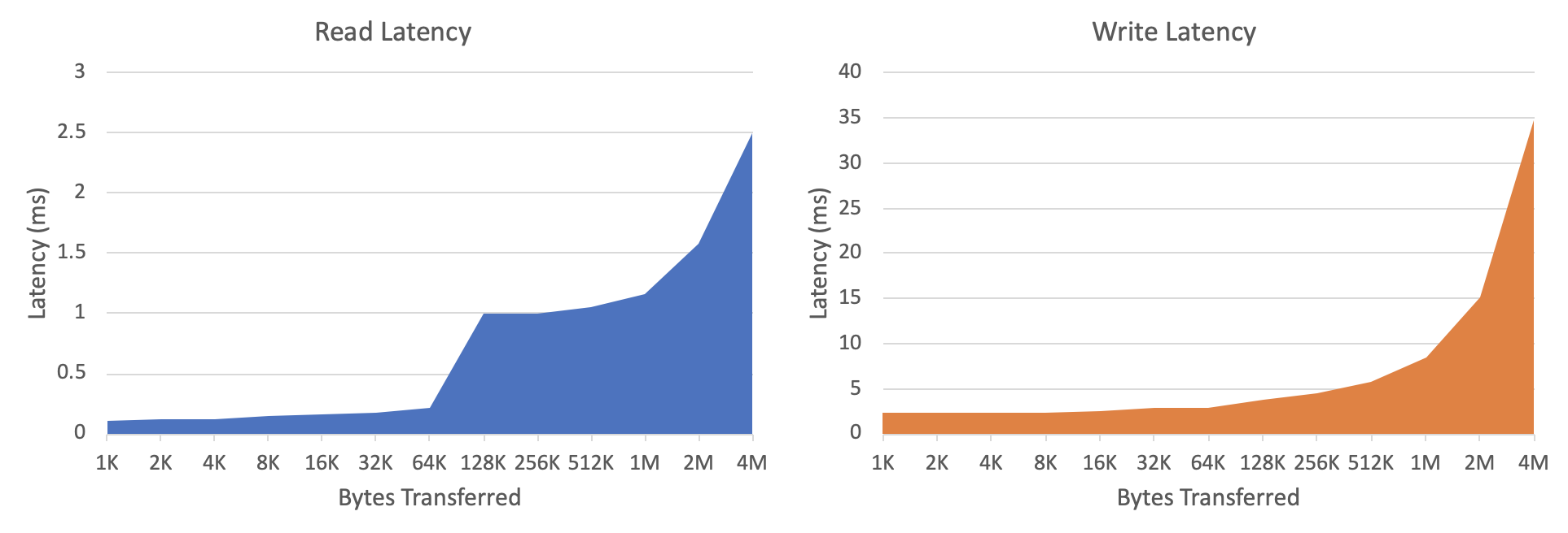
For this test, I executed many reads and writes from my disk using different I/O sizes (the number of bytes transferred per request). In the graphs above, the horizontal axis shows this I/O size, and the vertical axis shows the average latency (time to execute the transfer) for each I/O size in milliseconds.
Conventional wisdom says the time it takes to read or write data is proportional to how much data you want to read or write; if this were true, we would expect to see the latency grow exponentially in these graphs, because the horizontal axis grows exponentially (it doubles at each point) …
.. and that is eventually what happens, but the left side of each graph is roughly flat. This means, on average, the time it took to transfer 1 KB of data is about the same as it took to transfer 32 KB of data. (How could that be? This happens because there’s a fixed cost of setting up a disk I/O operation, which dominates the cost of actually reading/writing data unless you’re trying to read or write a lot of data.)
The conclusion, then, is that it’s okay to read a few kilobytes of extra data any time we only need a handful of bytes from disk. (If you think about it, this ought to play nicely with the caching strategies we mentioned above, eh?)
Access Counts (Constants Matter!)
Let’s take another look at the latency table from earlier, but this time let’s use the latencies to figure out how many ‘things’ we can do with each device per second:
| Device | Latency (Actual) | Operations / Second |
|---|---|---|
| CPU | 0.4 ns | 2,500,000,000 |
| Memory | 100 ns | 10,000,000 |
| Disk (SSD) | 50-150 μs | 6,700-20,000 |
| Disk (Rotational) | 1-10 ms | 100-1,000 |
| Network Request | 65-141 ms | 7-16 |
(All I did here was invert each latency — for example, there are 2.5 billion 0.4-ns intervals per second.)
The key thing to notice is that disks don’t give you all too many operations per second to work with, especially at the lower end (slower SSDs / rotational disks). Even if our map data structure has good big-$O$ performance, the absolute number of disk reads/writes is also important — if every client request causes us to do a few dozen disk operations, we’ll exhaust the disk’s throughput pretty quickly.
Evaluating our Data Structures
Putting together everything we just learned about disk hardware performance, here’s how we can summarize the design criteria that we want to design our map data structure around:
Say we’re storing small key/value pairs (say, around 100 bytes each).
Our map data structure should minimize the number of individual disk accesses …
… even if that means each operation transfers more data than strictly needed (up to a limit).
And, we plan to cache portions of this data structure in memory to exploit spatial and temporal locality in the client’s workload
So, how do hash tables and binary trees stack up?
Hash Tables
TODO scrambling the keys destroys any inherent spatial locality in the data structure. But we can’t not scramble the keys, or we’ll get more frequent collisions and worse performance
TODO and on top of that, there’s also no bound to how many disk accesses a single query might require. Sure it’s usually just one disk read, which is great, but worst case collision handling can lead to lots of disk accesses.
TODO so we don’t really like these
Binary Trees
TODO now this feels like a step in the right direction: at least the data structure is sorted right? Wrong! The links between nodes might provide us with a logical sort order, but on disk the nodes are scrambled around anyways. (Diagram showing the same scrambling pattern as the hash table, except now there’s a sentinel value labeled ‘root of tree’ and we add a bunch of inter-node arrows linking everything up. Showcase this side by side with the same ‘logical’ tree diagram as before.)
TODO these also have a real problem in terms of access counts! Consider a tree with 1 million elements: $\log_2(1,000,000) \approx 20$ disk accesses per read, which on a rotational disk means $20 \times 10 ms = 200$ ms per read. That means a single disk serving a binary tree-based index could only serve a whopping 5 requests per second — talk about cost-inefficient!
What Did We Learn?
TODO we want a sorted data structure, so that there’s inherent spatial locality in the map itself
TODO we want the items in this data structure to be sorted even on disk, so we can ‘over read’ and cache the results
TODO and finally, we want to minimize the number of disk accesses needed to read an item
TODO and it turns out there’s a data structure that does a fairly good job at all of these …
B-Trees
TODO
Okay, so we did a better job motivating how we’re going to get from binary trees to b-trees, which means now we can start to spell it out.
Basically, what I want to say is, start by noticing you can binary search a binary search tree by traversing it, but you can also binary search an array. What if our key value map was a gigantic array?
Problem: Updates might require rewriting all data on the disk, holy cow that’s slow
Oh yeah, that binary tree structure was helping us on insert
Okay, here’s the size observation: writing a ~4-16K batch of items is about as fast as writing a single item. Reading a 4-16K batch of items is about as fast as reading a single item. So what if we ‘smooshed’ the binary tree down into 4-16K runs of sorted items? (Diagram.)
And that’s precisely the core idea behind a b-tree!
Intuitively, the basic idea of a b-tree is to start with a binary search tree and ‘smoosh’ it down, kind of like this:
Diagram
Another way to think of this is making a binary tree ‘wider’ — whereas a binary tree has two children per node, a b-tree is an ‘$N$-ary’ tree with $N$ children per node (where $N$ is often in the hundreds). Typically, we pick a b-tree node size between 8 and 64 kilobytes, and stuff in as many key/value/child pairs as will fit.
To search a b-tree, we first read the root node from disk. We then search that node’s items array looking for either the item we want, or a gap between two items where our item would appear. In the latter case, we follow the child pointer to another node, which we then read from disk and search in the same way, recursively:
Diagram
We’re fundamentally still binary-searching a sorted collection as a tree, so the search complexity of our map is still $O(\log N$). However, since there are hundreds of items per node, there are hundreds times fewer nodes in a b-tree than there would be in a binary search tree with the same items. This saves us a lot of disk reads during searches.
Constructing a b-tree is a little more involved, but nothing we can’t handle. Wikipedia has a pretty good writeup if you’re curious about learning more.
Nice Properties of B-Trees
Compared to binary search trees, what nice properties do we get by ‘smooshing’ the tree down into a wider, shallower structure with large nodes?
The main advantage is making it almost trivial to build an in-memory cache that exploits both spatial and temporal locality. All we need to do is cache a copy of each b-tree node we’ve accessed recently: if the client comes queries a nearby key soon, chances are very good that key is in the b-tree node we just cached, so we can serve the query from the cached node with no disk reads.
Even better, reading a b-tree’s large nodes is ‘free’ compared to reading a binary search tree’s very small nodes, because the time it takes to read a handful of bytes from a disk is the same as it takes to read a handful of kilobytes — remember these graphs?
Finally, even if we don’t have the requested data in our cache, the very high branching factor of a b-tree keeps it shallow; for example, if you had a million items in a b-tree with 256 items per node, your tree would only have three levels, which means even if your cache were empty, you would only need to execute 3 disk reads to serve a client query (compared to 20 for binary trees, as we estimated earlier).
In practice, though, you’d basically never execute all three of those disk reads, because there’s an extremely good chance you cached some of the internal nodes already. For example, as long as you’ve queried any part of the tree recently, you already have the root node cached; that’s one less disk read you need.
The Ubiquitous B-Tree
For disk query performance, it’s hard to beat a b-tree, which is why they’re used across all sorts of data stores, from file systems to databases to caches and more. Much work has gone into optimizing b-trees, and there are many variants (the Wikipedia article on b-trees includes a nice overview of the different variants people have come up with).
But, for now, let’s get back to our key/value store.
Let’s Build a Key-Value Store
Now that we have a good data structure in mind, let’s build a key/value store on disk using a b-tree, and analyze its performance.
Complete the key-value store interface on top of this tree. Should be very easy.
Let’s Build a Database
This was originally written before we refactored the post to describe a generic ‘key/value store’ first, so this section may need some redrafting.
Overview showing what a database table looks like, with a diagram
We can decompose a row into a key-value mapping by examininng the table schema
Diagram
A table, then, is a sorted array of this key-value mapping.
So then the obvious approach is to store the database as a b-tree of rows.
Diagram showing the example table on one side, the same rows in a b-tree on the other side
Each record is a row, which can be decomposed into both a key and a value as described above.
Let’s look at how common queries work
- Insert - show how this is a row insert
- Select - with a single key
- Select - with a range of keys
- Delete -
To complete your database now all you need is a transaction manager (which locks ranges of keys that are being operated on, to provide isolation) and a query parser (giving users an interface to your database)
Huzzah! We solved storage systems … or did we? How do you handle data that’s larger than what can fit in a single b-tree node?
This is the purview of a different, but closely related kind of storage system . . .
File Systems
Databases vs file systems: similar in principle, differ in target workloads. Databases optimize for large numbers of relatively small ‘records’ (rows), whereas file systems optimize for smaller numbers of relatively larger ‘files.’ Plenty of overlap.
Although file systems are not tied to b-trees as closely as databases usually are, many modern file systems use b-trees ubiquitously (such as btrfs on Linux, ReFS on Windows?, AFS on macOS? Others worth mentinoinng?)
Naming Hierarchy
Very quick overview of files and directories. Show how this is basically the database problem all over again, and how b-trees are a good fit
File Contents and Handling Large Items
The database design assumed many small key and value records, but files can get pretty darn big: the name is still a small key, but the value (file contents) can be gigabytes to terabytes in size. You can’t stick these file contents in your b-tree because they’re often much larger than any particular node of your b-tree.
Do we need to throw away our system and start over with something new? How does a file system handle these large items?
Think about the interface a disk provides, and fundamentally how a b-tree is laid out on disk
Diagram showing a byte array, b-tree nodes in that byte array pointing to each other
Idea: drop data anywhere on disk you have room to put it, then use a b-tree record to point to the data by its disk address:
Diagram
Disk Allocation
Explore the problem of allocating space on a disk, both for allocating blocks of space for file contents and for allocating blocks of space for b-tree nodes. Note that a b-tree can even be used for this.
Mention fragmentation, this is more than just a data structures problem, very similar to writing a memory allocator since disks are very similar to memory
When to Build Storage Systems
Salvage some of the content from the old ‘optimizing and tradeoffs’ section. The main argument is that every system optimizes for certain workloads and the expense of being worse at other workloads, and sometimes you have a workload that nobody has ever optimized for — and that’s when you break out this theory and go build your own system.
Where To Next
Other concerns like resiliency (checksums), concurrency control
New unconventional types of storage devices which meld performance aspects of disks and memory
Append-only stores and the unique challenges they pose
Distributed stores and the unique challenges they pose
Additional Reading
Plug DDIA